Adaptive (Asynchronous) Method

The adaptive_asha search method employs an Asynchronous version of the Successive Halving Algorithm (ASHA), which is suitable for large-scale experiments with hundreds or thousands of trials.

Quick Start

Here are some suggested initial settings for adaptive_asha that typically work well.

Search mode:

• mode: Set to standard.

Resource budget:

• time_metric, max_time: The name of the “time” metric and the maximum value it will take for a trial that survives to the end of the experiment (see Training Units). Note that the searcher will expect this metric to appear in validation metrics reported by the model. This quantity is domain-specific and should roughly reflect the number of minibatches the model must be trained on for it to converge on the dataset. For users who would like to determine this number experimentally, train a model with reasonable hyperparameters using the single search method.

• max_trials: This indicates the total number of hyperparameter settings that will be evaluated in the experiment. Set max_trials to at least 500 to take advantage of speedups from early-stopping. You can also set a large max_trials and stop the experiment once the desired performance is achieved.

• max_concurrent_trials: This field controls the degree of parallelism of the experiment. The experiment will have a maximum of this many trials training simultaneously at any one time. The adaptive_asha searcher scales nearly perfectly with additional compute, so you should set this field based on compute environment constraints. If this value is less than the number of brackets produced by the adaptive algorithm, it will be rounded up.

Details

Conceptually, the adaptive_asha searcher is a carefully tuned strategy for spawning multiple ASHA (asynchronous successive halving algorithm) searchers, themselves hyperparameter search algorithms. ASHA can be configured to make different tradeoffs between exploration and exploitation, i.e., how many trials are explored versus how long a single trial is trained for. Because the right tradeoff between exploration and exploitation is hard to know in advance, the adaptive_asha algorithm tries several ASHA searches with different tradeoffs.

The configuration settings available to Determined experiments running in adaptive_asha mode mostly affect the ASHA subroutines directly. The mode configuration is the only one affecting the decisions of the adaptive_asha searcher, by changing the number and types of ASHA subroutines spawned.

The first section here gives a description of the synchronous version of ASHA called successive halving. The second section discusses the motivation for the asynchronous promotions used by ASHA. The third section describes why you would choose adaptive_asha over plain asynchronous_halving. The final section and conclusion is a set of FAQs regarding adaptive_asha.

ASHA

At a high level, SHA prunes (“halves”) a set of trials in successive rounds we call rungs. SHA starts with an initial set of trials. (A trial means one model, with a fixed set of hyperparameter values.) SHA trains all the trials for some length and the trials with the worst validation performance are discarded. In the next rung, the remaining trials are trained for a longer period of time, and then trials with the worst validation performance are pruned once again. This is repeated until the maximum training length is reached.

First, an example of SHA.

• Rung 1: SHA creates N initial trials; the hyperparameter values for each trial are randomly sampled from the hyperparameters defined in the experiment configuration file. Each trial is trained for 1 epoch, and then validation metrics are computed.

• Rung 2: SHA picks the N/4 top-performing trials according to validation metrics. These are trained for 4 epochs.

• Rung 3: SHA picks the N/16 top-performing trials according to validation metrics. These are trained for 16 epochs.

At the end, the trial with best performance has the hyperparameter setting the SHA searcher returns.

In the example above, we generalize “halving” with a field called divisor, which determines what fraction of trials are kept in successive rungs, as well as the training length in successive rungs. In this example, time_metric would probably be “epochs” and max_time would be 16, since the maximum time a trial is trained for is 16 epochs.

In general, SHA has a fixed divisor d. In the first rung, it generates an initial set of randomly chosen trials and runs until each trial has trained for the same length. In the next rung, it keeps 1/d of those trials and closes the rest. Then it runs each remaining trial until it has trained for d times as long as the previous rung. ASHA iterates this process until some stopping criterion is reached, such as completing a specified number of rungs or having only one trial remaining. The total training length, rungs, and trials within rungs are fixed within each SHA searcher, but vary across different calls to SHA by the adaptive algorithm. Note that although the name “SHA” includes the phrase “halving”, the fraction of trials pruned after every rung is controlled by divisor.

Why Asynchronous Halving?

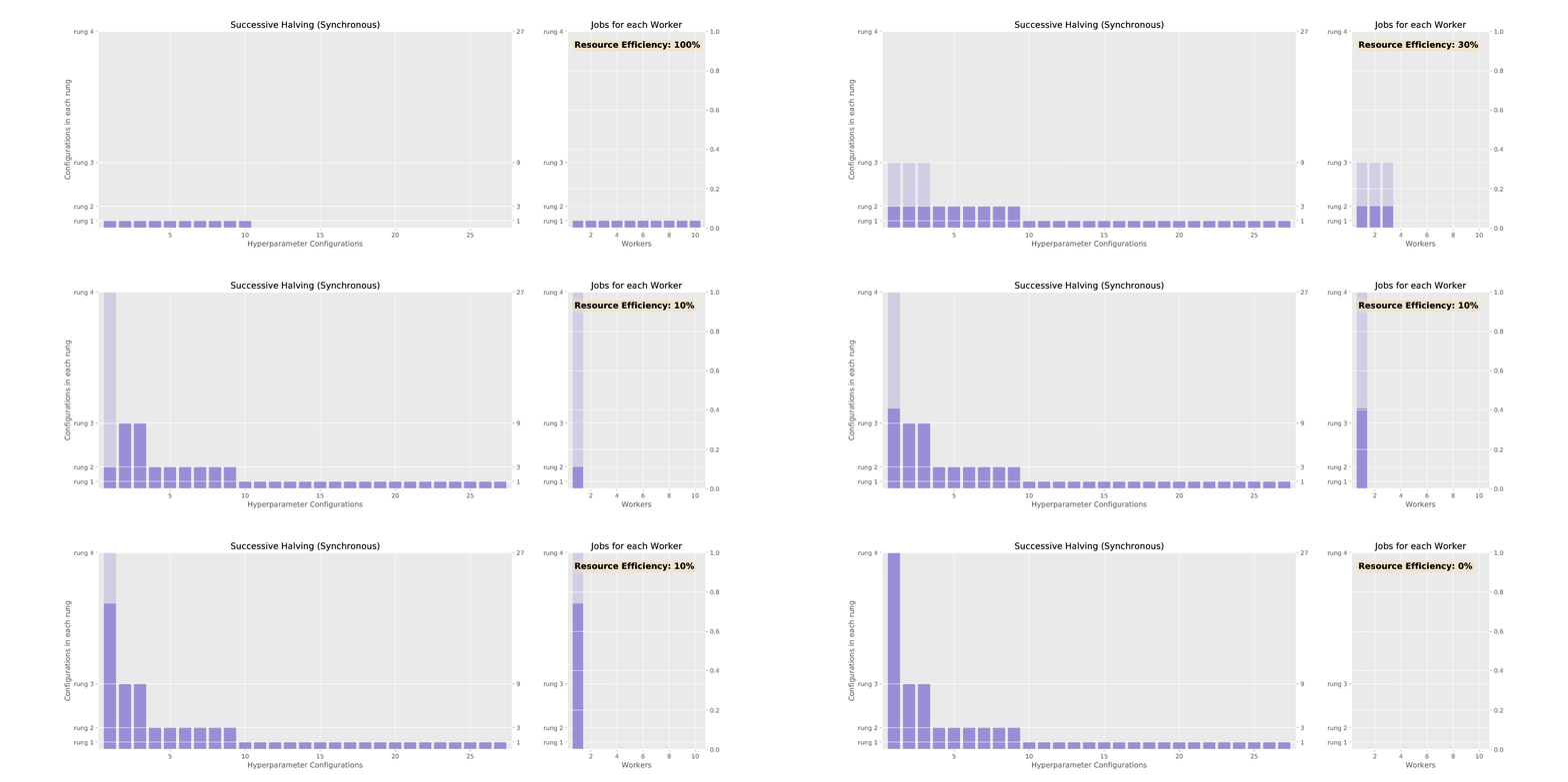
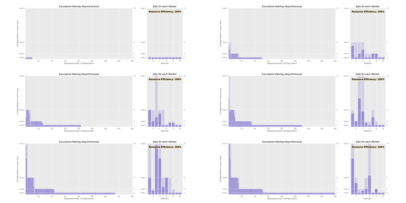
Successive halving (SHA) promotes hyperparameter configurations synchronously, waiting for each rung to complete before performing any promotions. This allows the algorithm to have complete information about all trials at the time of promotion, but it results in underutilized nodes waiting on completion of validation steps for other configurations. ASHA, asynchronous successive halving, asynchronously promotes trials when it has the minimum information required to make a decision in order to maximize compute efficiency of the searcher. In contrast to SHA which initializes all trials in the bottom rung at the outset, ASHA will continuously add trials to the bottom rung until the desired number of trials is reached.

See the difference in asynchronous vs. synchronous promotions in the two animated GIFs below:

Adaptive over ASHA

The adaptive algorithm calls ASHA subroutines with varying parameters. The exact calls are configured through the choice of mode, which specifies how aggressively to perform early stopping. One way to think about this behavior is as a spectrum that ranges from “one ASHA run” (aggressive early stopping; eliminate most trials every rung) to “searcher: random” “multiple ASHA runs, some of which will not early stop and others will early stop later” (try some without early stopping; initialized trials may be allowed to run to completion).

On one end, aggressive applies early stopping in a very eager manner; this mode essentially corresponds to only making a single call to ASHA. With the default divisor of 4, 75% of the remaining trials will be eliminated in each rung after only being trained for 25% the length of the next rung. This implies that relatively few trials will be allowed to finish even a small fraction of the length needed train to convergence (time_metric, max_time). This aggressive early stopping behavior allows the searcher to start more trials for a wider exploration of hyperparameter configurations, at the risk of discarding a configuration too soon.

On the other end, conservative mode is more similar to a random search, in that it performs significantly less pruning. Extra ASHA subroutines are spawned with fewer rungs and longer training lengths to account for the high percentage of trials eliminated after only a short time. However, a conservative adaptive search will only explore a small fraction of the configurations explored by an aggressive search, given the same budget.

Once the number and types of calls to ASHA are determined (via mode), the adaptive algorithm will allocate training length budgets to the ASHA subroutines, from the overall budget for the adaptive algorithm (user-specified through budget). This determines the number of trials at each rung (N in the above ASHA example).

FAQ

Q: How do I control how long a trial is trained for before it is potentially discarded?

The training length is guaranteed to be at least max_time / 256 by default, or max_time / divisor ^ max_rungs-1 in general. It is recommended to use records or epochs as your time_metric if your batch size is not constant across all trials, to ensure each trial trains on the same amount of data.

Q: How do I make sure ``x`` trials are run the full training length (``max_time``)?

The number of initial trials is determined by a combination of mode, max_trials, divisor, max_rungs, max_time and bracket_rungs. Here is a rule of thumb for the default configuration of max_rungs: 5 and divisor: 4, with mode: standard and a large enough max_trials:

• The initial number of trials is max_trials.

• To ensure that x trials are run max_time, set max_time high enough for the brackets with their halving rate (the divisor) to allow x trials to make it to the final rungs. This can be viewed by the command describe below.

A configuration setting that meets set goals can be found by trial and error. The command

det preview-search <file_name.yaml>

will display information on the number of trials versus training length for the configuration specified in file_name.yaml.

Q: The adaptive algorithm sounds great so far. What are its weaknesses?

In our experience, early-stopping works well across a variety of deep learning models. However, there may be some search spaces in which early-stopping underperforms simple random search. This can happen if model complexity varies drastically in a search space leading to different converge rates or if the search space contains hyperparameters that are strongly correlated with training length.